The global Opportunity Mapping tool is the first to cross-map ecosystem distribution with human exposure to hazards at a global scale. It shows areas where ecosystem management could be used to protect the greatest number of people globally.
It should be noted that the cross mapping of ecosystem coverage and hazard exposure consists simply of the quantification of the intersection of a hazard exposure with an ecosystem coverage. These outputs do not include an analysis of capabilities for action at a local scale (e.g. restoration or protection activities cannot be implemented wisely in urban areas).
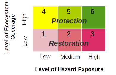
The EcoDRR classification scheme applied to the global and country level grid cell layer is based on six classes scheme.
In areas where ecosystem coverage is low, but exposure to hazards is high, ecosystem restoration can provide an opportunity to reduce disaster risk.
Where ecosystem coverage is high and exposure is also high, ecosystem protection provides an opportunity to reduce risks to the population, while loss of the existing ecosystem may lead to higher exposure of the population.
Data used
The reference Grid layer
The reference layer which will integrate the opportunity mapping and the spatial statistics is a vector grid of equal area cells. Equal area cells allow generating statistics that are comparable at global scale, even in term of absolute numbers (i.e. physical exposure to natural hazards). The present grid layer has cells of approximately 100 km2.
Population dataset
A new population dataset is used for physical exposure calculation: Population density map (HRSL-GSHL) 2022.
The layer integrates data from the High Resolution Settlement Layer (HRSL) - META (originally Facebook), the Global Human Settlement Layer (GHSL) - JRC, and the national population count for 2018 reported on the World Population Prospects 2019. Pixel counts are recalculated for 2022 based on the country population data reported for 2022 by the World Population Prospects 2019.
Ecosystems
Before being subsequently aggregated on the reference grid, the four ecosystems taken into consideration are processed at 0.01 degree resolution using a raster of real area.
Forest
The updated forest coverage is derived from the The MODIS Terra and Aqua Combined Land Cover Type Version 6 (MCD12Q1). The year 2020 of the Land Cover Type Yearly L3 Global 500m is used. Among the FAO-LCCS2 land use layer, two are selected: Open Forests: tree cover 10-60% (canopy >2m) and Dense Forests: tree cover >60% (canopy >2m). The main advantage of using MODIS Land Cover Type Dataset is its yearly update.
Mangrove
The Global Mangrove Watch layer shows a better global coverage and replaces the former WCMC Global Distribution of Mangroves
Coral reefs
The last version of WCMC Global Distribution datasets is used for coral reef: This dataset shows the global distribution of coral reefs in tropical and subtropical regions. It is the most comprehensive global dataset of warm-water coral reefs to date, acting as a foundation baseline map for future, more detailed, work.
Seagrass
The last version of WCMC Global Distribution datasets is used for seagrass
The quality of ecosystem in a 100 km2 grid cell is expressed as its area percentage, considering cell land area for forest, ocean area for coral reef and sea grass, and total cell area for mangroves. This value is used for the final Opportunity Mapping Tool classification.
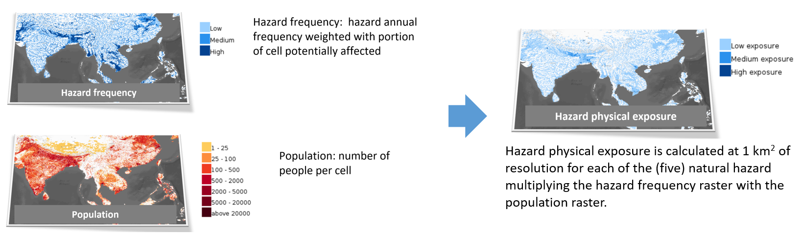
Natural hazards frequency
Physical exposure was calculated for each natural hazard multiplying the hazard frequency raster with the population raster. Flood hazard model having various return period layers, the final physical exposure is the sum of each single physical exposure.
The physical exposure in the reference grid (100 km2 grid cell) is the sum of the included physical exposure raster cells. This number is used for the final Opportunity Mapping Tool classification.
Landslide
The landslide hazard is separated in two categories: landslides triggered by earthquakes or precipitations. In our case, the final frequency raster is the sum of both hazard annual frequencies. The postulate being that a pixel affected by an earthquake landslide event could still be affected by a precipitation landslide event during the same year and somewhere else in the pixel. Source GAR 2009, / Global Risk Data Platform Landslides
Tropical cyclone (wind)
In the case of Tropical cyclones, annual frequency raster is calculated with the “fixed wind speeds” dataset, using the 30 m/s mean wind speed return period estimates. The six regions layers are merged together and resampled to match the required 0.01 degrees input datasets. Source 4TU.ResearchData
Tropical cyclone (surge)
To generate the new Cyclone surge layer, the original point dataset water height values corresponding to each available return period are interpolated alond the coastline.To account for surface roughness that reduces the water level inland, the resulting water height is decreased with distance away from the coastline using a recommended attenuation factor of 0.5 m/km. Pixels values higher than land elevation are conserved to generate each return period water height layer. The final storm surge frequency layer is obtained by summing each layer return period value. Source 4TU.ResearchData
Tsunami
Source: GAR 2015, / Global Risk Data Platform Tsunami
River flood
Source: GAR 2015, / Global Risk Data Platform Floods
Methodology
For a complete and detailed methodology please refer to: Chatenoux et al. (2017) and Herold (2022)
Physical exposure
Physical exposure was computed by multiplying the frequency of occurrence of a given hazard in any location by the population of that location (both datasets are in raster format).
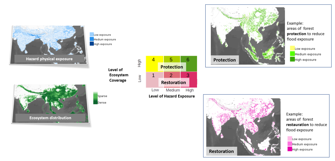
Hazard exposure/Ecosystem coverage combinations (cross-mapping)
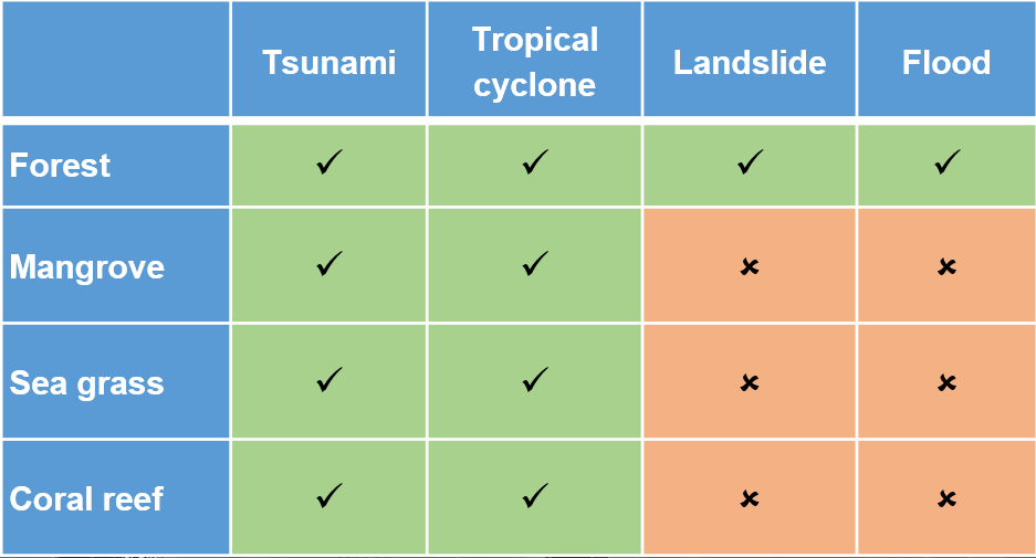
The next step consisted of combining a given hazard exposure with a given ecosystem cover. Each ecosystem type can effectively reduce exposure to a particular set of hazards, but not all. For example, coral reefs can reduce exposure to tsunami and storm surge, but are not effective buffers against winds, landslides or flooding that originates inland. Therefore only the relevant hazard types were cross-mapped with each ecosystem type.
Then, the overlay operation determines the proportion of ecosystem coverage within each cell. Finally, a classification is applied for the output layers: restoration opportunities are identified for areas with low ecosystem coverage, and protection opportunities for areas with higher ecosystem coverage.For each considered combination of hazard physical exposure and ecosystem, the six classes are obtained by finding the tertiles of physical exposure and the median of ecosystem datasets.
At global scale, these statistics are done on a selected sample of grid cells that include positive values for both physical exposure and ecosystem percentage area.
The country level classification is obtained the same way, but on a selected sample of cells overlapping the considered country area. It generates tertiles and median based respectively on each country hazard exposure and ecosystem area sample range. It creates a classification that better suits the national conditions of both parameters. This classification also allows for an overview within the country. It has been used for the graphs in the statistical data section of this platform
Two additional classes allow to display information about special cases:
- Value 11: attributed to cells including hazard occurrence and ecosystem area, but with no population.
- Value 12: attributed to cells including hazard occurrence and population (physical exposure), but no ecosystem area.
Conclusions
Currently the analysis focuses on each cell as an isolated element, however neighbouring cells possibly have an influence on each other’s exposure level to hazards (depending on topography, type of hazard and ecosystem). Future iterations of the tool could explore an analysis of the influence of neighbouring pixels on exposure and ecosystem coverage
There are two noteworthy issues to take into consideration when using the tool.
First, the percentage of urban cover is not estimated. This creates an artefact whereby built-up areas may be highlighted as areas with high ecosystem restoration potential even if this in not practically feasible nor realistic as land for restoration may not be available.
Second, climatic zones (typically highly arid zones) were not included in assessing the suitability of ecosystem-based approaches as these are not areas where vegetation exist naturally and/ or cannot easily be detected at the 10 x10 km scale. Because of these limitations and its coarse spatial resolution, the global products should be used as an awareness and first screening tool for Nature-based approaches to disaster risk reduction and not for planning purposes, which require higher resolution data sets
References
Chatenoux, B., Peduzzi, P. (2007): Impacts from the 2004 Indian Ocean Tsunami: analyzing the potential protecting role of environmental features, Natural Hazards, 40:289–304. Impacts from the 2004 Indian Ocean Tsunami.pdf
Chatenoux, B. and Wolf, A. (2013): Ecosystem based approaches for climate change adaptation in Caribbean SIDS. UNEP/GRID‐Geneva and ZMT Leibniz Center for Tropical Marine Biology, pp.64. CaribbeanSIDS.pdf
Chatenoux, B., Peduzzi, P., Estrella, M. & Bayani, N. (2017): Promoting Improved Ecosystem Management in Vulnerable Countries for Sustainable and Disaster-Resilient Development, UNEP/GRID-Geneva & UNEP/PCDMB PCDMB UNIGE ECO-DRR 2016 - Technical Report.pdf
Herold, C. (2022): Eco-DRR Opportunity Mapping Tool Update, Technical note, UNEP/GRID-Geneva EcoDRRmapping_technical_report june-2022.pdf
Sudmeier-Rieux, K., Nehren, U., Sandholz, S. and Doswald, N. (2019): Disasters and Ecosystems, Resilience in a Changing Climate - Source Book. Geneva: UNEP and Cologne: TH Köln - University of Applied Sciences Source Book.
UNEP (2010): Risk and Vulnerability Assessment Methodology Development Project (RiVAMP), Linking Ecosystems to Risk and Vulnerability Reduction The Case of Jamaica, United Nations Environment Programme, Geneva, 99 p. RIVAMP report
UNDP (2004): Reducing Disaster Risk: a challenge for development, United Nations Development Programme, Bureau for Crisis Prevention and Recovery, New York, NY 10017, 146 p.
UNISDR (2009, 2011, 2013 and 2015): Global Assessment Report (GAR) on Disaster Risk Reduction, United Nations International Strategy for Disaster Reduction, United Nations, Geneva, Switzerland. GAR reports